Outliers in Data, Emphasis in Data Science.

Outlier – The Enemy under wraps

Outlier: I always like to think an outlier as Shashi Tharoor placed between general English-speaking group. He would really stand out, in the way he speaks English.Well, Shashi Tharoor will be an outlier in most groups. 

 Outlier is a point or observation that differs significantly from the from the rest of the data. In a distribution of variable, it is that value that so far away from the usual values in that variable. It is also commonly referred to as Anomaly. 

“An outlier is an observation which deviates so much from the other observations as to arouse suspicions that it was generated by a different mechanism.” 

Example: 10,12, 13 ,15,16, 17, 18, 23, 297. 

297, is an outlier. 

Outliers are also referred to as abnormalities, discordants, deviants, or anomalies. Outlier detection is a common practice in credit card fraud analysis, medical diagnosis, intrusion detection etc. 

Outlier can be a result of error in measurement arising due to human error mostly. It can sometimes occur due to sample coming from a entirely different population and sometimes it just a rare event.

That brings me to an important point, that it depends upon the domain as to what constitutes an abnormal behavior in the data. In a medical domain, the threshold is different as opposed to a banking domain. It is important to understand what is normal, what is noise and what is a extreme behavior.

There are various outlier detection algorithms and techniques. We will discuss some of the techniques used in feature engineering while building a machine learning model.

The Famous 3-sigma rule – Holy Trinity of statistics

This rule comes from the “Godly” distribution which is normal distribution.

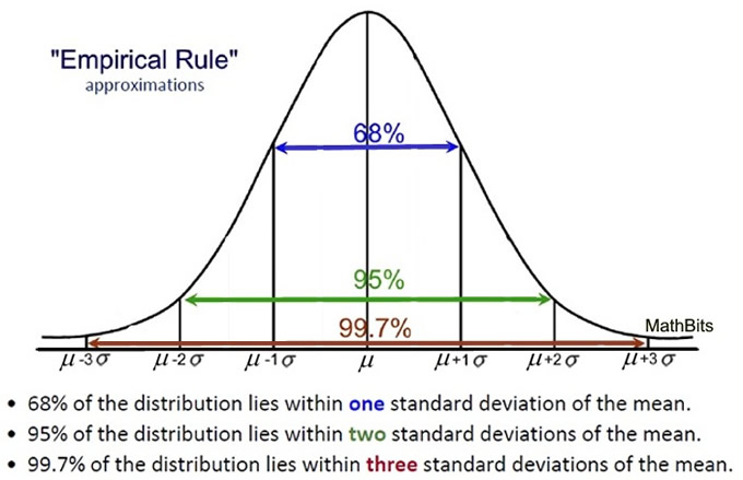
A normal distribution is a very common probability distribution that approximates the behavior of many natural phenomena. A variable is “normally distributed” when most of the observations aggregates around its mean in a symmetric fashion. Values become less and less likely to occur the farther they are from the mean.

As we have established, values become less and less likely as we go further away from the mean and that is where the answer to the problem exist. So variable should follow 68-95-99.7 distribution it is deemed normal, the moment it does not follow this 68-95 rule you can sense an anomaly.

We can say that any value that is -4 standard deviation away from the mean and +4 standard deviation away from the mean would be considered as an outlier. There is more to it.

You are far away but measurably close – The Z-score

Z-score is the number of standard deviation away a data point is from the mean. The basic idea of this rule is that if X follows a normal distribution, N (µ, σ2), then Z follows a standard normal distribution, N (0, 1), and Z-scores that exceed 3 in absolute value are generally considered as outliers.

µ = population mean, σ2 = variance

If you see both the aforementioned rules to screen out outliers, they almost tell the same thing with different parameter. Each method has their own limitation for example z-score method depends upon sample size. what is the impact if the sample size is small or dataset is really small? There are many other things to debate.

MAD(median absolute deviation) RULE: Its is significantly not so mad

While statistics like mean and standard deviation are used to screen outliers, one needs to consider that they themselves are affected by outliers. Standard deviation is based on squared distances so extreme points on either side, exert their weight.

Median is a more robust statistic, it does not get affected by an outlier. For MAD, first, you calculate the median of the variable X and then subtract each observation of X from the median, take their absolute values and then take the median from those values.

The Rule is simple: All you need to do after you have median standard deviation is to multiply it by 2, 2.5, or 3. Depending on how conservative you’re feeling. Then add and subtract the resulting value from the median. Any observation falling outside of this window are outliers. This method is preferred over normal standard deviation method.

There is an extension to this rule. Attaching a Consistent Estimator.This modification will ensure that for large samples the MAD provides a good estimate of the standard deviation (more formally, the MAD becomes a consistent estimator of the population standard deviation). It is 1.4826.

The Box Plot Method: The box with wizard sections

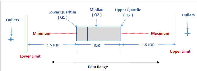
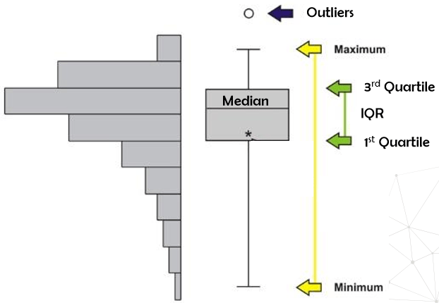
For Skewed distribution, the general rule is to calculate quantiles and interquartile range. The quantiles are values that divide the distribution such that there is a given proportion of observations below the quantile. For example, the median is a quantile. The median is the central value of the distribution, such that half the points are less than or equal to it and half are greater than or equal to it.

IQR = 75th Quantile – 25th Quantile

Within the interquartile range, we will find 50 percent of the observation. Once you calculate the interquartile range, we need to find the limits beyond which an observation can be considered as an outlier. Now the top limit is given by 75th Quantile + IQR × 1.5 and the lower limit is given by 25th Quantile – IQR × 1.5. There are instances where we are interested in extremely unlikely events there we multiply the IQR with 3 than 1.5.

for skewed distribution the boxplot looks slightly different. the interquantile range is concentrated where majority of the values are concentrated the median is towards the opposite side of the tail and whiskers are asymmetrical. This helps capture the distribution of skewed variable.

LOF (Local Outlier Factor) method: The one where density matters

This method is based on the idea of nearest neighbors. If you have a little idea about a simple k-nearest algorithm of machine learning, you should be able to understand this.

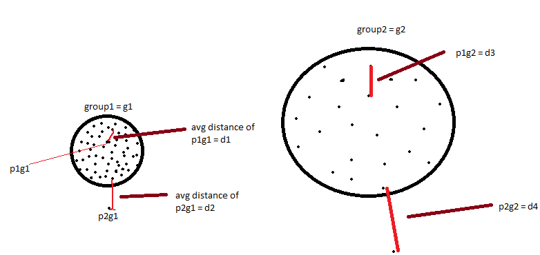
Imagine there is variable X and its observations are such that they form two groups when you plot them, one where the observations are densely populated, we will call that group as g1. Another group we call it g2 where the observations are sparsely populated.

Lets dive into how it works.

1. K in K-nearest neighbor is the number of neighbors. We will assume K=3, which means we will pick three nearest neighbor.
2. Suppose you have 50 points in group 1 and 50 points in group 2.
3. For each point we will first encircle the 3-nearest neighbor and calculate the avg distance from those nearest neighbor. We will do this for each point.
4. We also have two outlier p2g1(p2 in the group 1) and p2g2(p2 in the group 2).
5. We will also calculate the average distance from these point the same way we did for the other points.
6. After getting all the distances we will sort the distances. Once we sort the distance we will pick the one the with highest average distance(this is across all groups) and that will be our outlier.
7. But the problem is with the point p2 of group 1. Though this is an outlier but since we are considering all the groups as one, it is not getting picked as an outlier, it is getting overshadowed by the distances of the sparser group that is group2.
8. So we need to bring in local density into picture to make sure that outlier gets picked correctly.

For that reason the local density is considered and LOF does exactly that. First we need to understand reachability distance and local reachability density.

Reachability Distance:

Reachability distance between (X,Y) is given max (k-distance(Y), dist(X,Y))

continue….

In computer performance, we’re especially concerned about latency
outliers: very slow database queries, application requests, disk I/O,
etc. The term “outlier” is subjective: there is no rigid mathematical
definition.